
I love those images that you can see nowadays online where some software automatically detects and annotates the objects it sees. Could that be done for astronomy projects? Say images or live streams of the Sun, Moon, or deep sky? It would be nice to automatically tag objects and help the viewer answer questions such as: what is this lunar crater named? where are the solar prominences? what deep sky object is this?
As a scientist, I am always eager to experiment with new features. Machine Learning (ML) is something I have always found exciting despite many algorithms working as black boxes, meaning that you cannot really tell why they work the way they do. The cool thing is that ML algorithms learn from examples just as the human brain does. If 20 or so years ago libraries for ML were insufficiently developed and you had to learn to code your own neural network for recognizing features (yes, I learned how to do that as a computer science student), nowadays ML libraries are ubiquitous and pervasive. It is even becoming accessible to non-ML specialists.
These past few days I finally got the chance of having a few days free for playing around with ML libraries and Python. As I am partially working on my remote observatory focusing on setting up the software for it (you can check my previous post on setting up a Pi4 board for remote telescope control) I decided to create a small script that uses my ASI120MC USB2.0 camera installed on my LUNT40 B600 solar scope to automatically classify in real-time or on prerecorded videos or images, features on the Sun’s surface (prominences, filaments, faculae, and sunspots).
If you are interested in running ASI120MC USB2.0 on the Pi4 check my Youtube video explaining my solution. I plan on testing the software on that board as well but for this post, I will explain how I got the whole thing working on my Windows 10 Lenovo Yoga 530 laptop.
Machine learning and related libraries
Let’s start with some requirements (download links are posted where applicable). The list contains the software versions I used, others could work as well.
- Python 3.7.9 (direct link to Python 3.7.9 Windows installer). Just download the installer .exe file and follow the instructions. Python comes with a utility called pip that you will need for installing the required libraries.
- Install the following using the pip command from a Windows terminal:
- Tensorflow 1.15.0 (machine learning platform)
pip install tensorflow==1.15.0 - Tf-slim
pip install --upgrade tf_slim - Keras 2.2.4 (neural network library that contains the algorithms we will use)
pip install keras==2.2.4 - Protobuf 3.20.3
pip install protobuf==3.20.3. Make sure to uninstall the existing one:pip uninstall protobufbefore - h5py 2.10.0
pip install h5py=2.10.10 - Pycocotools
pip install pycocotools - Lvis
pip install lvis - Numpy 1.19.5
pip install numpy==1.19.5
- Tensorflow 1.15.0 (machine learning platform)
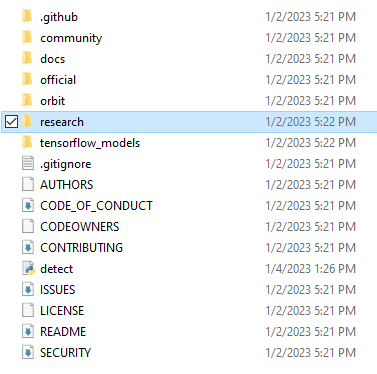
- Download and unzip the Tensorflow models from https://github.com/tensorflow/models (click on the green button called Code and then choose Download zip). I have unzipped mine in the Downloads folder. The model-masters folder should look like the below:
Preparing the training data
Skip to the Performing real-time feature detection section if you just want to use the model and not train your own!
The train the ML model to recognize various features on the Sun’s surface I first acquired images over the span of several months. The more the better, but unfortunately given the weather in the UK and my teaching commitments I could only get 14 days’ worth of data in .png format. So far by 9 August 2023 I gathered 37 days of data.
The images must be prepared for Tensorflow by annotating them and generating the necessary auxiliary files. I found this tutorial to be very helpful.
For labeling, I relied on LabelImg which can be also installed using pip install labelImg. The exe file will be available from the Python installation folder which is usually in the user’s AppData folder. In my case it is C:\Users\fmarc\AppData\Local\Programs\Python\Python37\Scripts. Do not change anything in the AppData folder unless you know what you are doing. It is a hidden folder where the applications are usually installed.
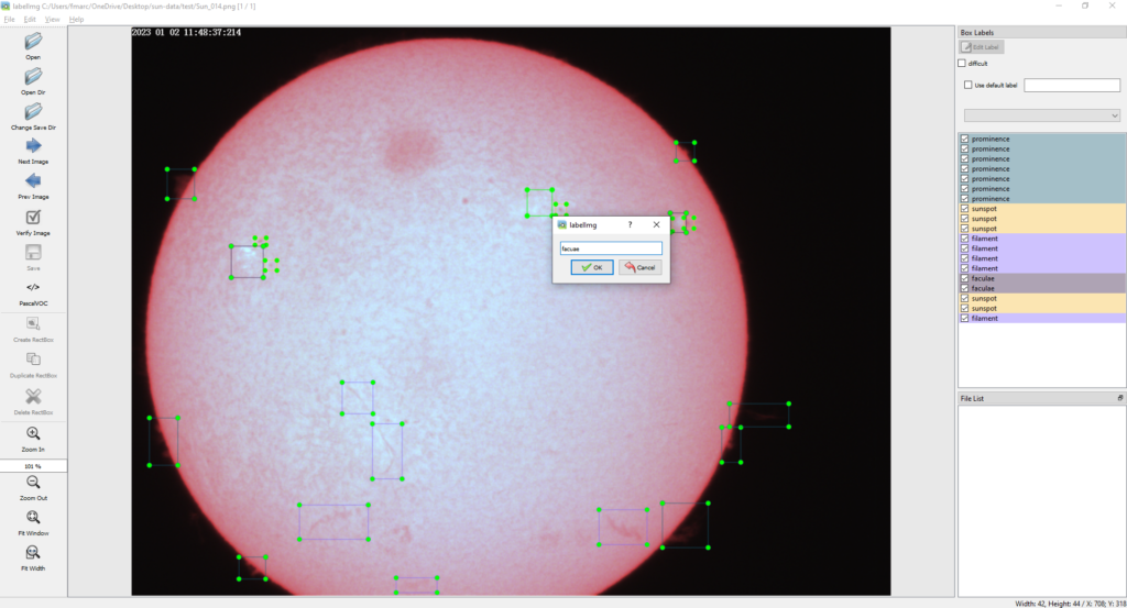
For me, double-clicking on its name and running it from there is easiest. Once the window opens go to Open or Open folder and start labeling your images by using the Create RectBox option. All buttons are found in the lefthand side menu. Once you add a box you can add the classes of your objects. In my case, I use four: prominence, faculae, filament, and sunspot. The image below shows an example:
It is best if you split your data into training, evaluation, and testing data. Create a separate folder for each. There is no best ratio but 80-10-10 percent is a good start. In my case, I had 14 images in total from which I used 12 to train the model and 2 to evaluate it. I did not use any images for testing as I plan on doing that on a live stream. The more the merrier and I plan on improving the model as I get more data. For labeling, I use unprocessed images to capture any artifacts from my camera. In fact, you can see the huge dust spot on the top part of the sun. Others are also present.
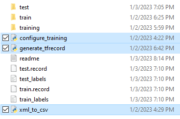
The process will generate XML files for each file you annotate. These must be transformed into TFRecords and a labelmap (.pbtxt) file for training our model. I have used several scripts found here. The three script files you must download and copy in the folder containing your annotated images are: configure_training.py, generate_tfrecord.py, and xml_to_csv.py. The main script that you will use is configure_training.py.
To make everything work I discovered that I had to add the following two lines:
sys.path.append('C:/Users/fmarc/Downloads/models-master/models-master/research')
sys.path.append('C:/Users/fmarc/Downloads/models-master/models-master/research/object_detection/utils')
just before these lines:
from object_detection.utils import ops as utils_ops
from object_detection.utils import dataset_util
which are found in the generate_tfrecord.py file, otherwise the script cannot find the imports. You must replace the path with your own pointing the research/ and research/object_detection/utils/ folders in the Tensorflow models you have previously downloaded.
Once this is done, create a training folder in the (see image above) and run the following two commands from a terminal to generate the required model files:
cd C:/Users/fmarc/OneDrive/Desktop/sun-data/
python configure_training.py -imageRoot C:/Users/fmarc/OneDrive/Desktop/sun-data/ -labelMap "faculae:1,prominence:2,sunspot:3,filament:4" -labelMapOutputFile C:/Users/fmarc/OneDrive/Desktop/sun-data/training/labelmap.pbtxt
Where –imageRoot points to the folder containing the images (should be the current folder), –labelMap contains our object classes, and –labelMapOutputFile contains the output folder where the .pbtxt file will be created. The process will also generate 4 more files in the current folder: test.record, test_labels.csv, train.record, train_labels.csv.
If all goes well you should see something similar to the below:
C:/Users/fmarc/OneDrive/Desktop/sun-data
Successfully converted xml to csv.
{'faculae': 1, 'prominence': 2, 'sunspot': 3, 'filament': 4}
Successfully created the TFRecords: C:/Users/fmarc/OneDrive/Desktop/sun-data/train.record
{'faculae': 1, 'prominence': 2, 'sunspot': 3, 'filament': 4}
Successfully created the TFRecords: C:/Users/fmarc/OneDrive/Desktop/sun-data/test.record
Training a predefined model
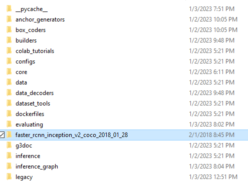
For training, I chose a predefined model as explained here. The model was faster_rcnn_inception_v2_coco and the archive can be downloaded from https://github.com/tensorflow/models/blob/master/research/object_detection/g3doc/tf1_detection_zoo.md. You can use other models if you want, the only reason I picked this one is that most online tutorials use it. The method applied here is actually called transfer learning as it involves improving an existing model trained on a different dataset to recognize your own labels.
The archive should be unzipped and the entire folder copied to the /models-master/research/object-detection/ folder as seen below:
Next, copy the faster_rcnn_inception_v2_pets.config file from object_detection/samples/configs/ folder to the object_detection/training/ folder (create it if not present). The file should be updated to reflect the configuration for this use case. A full file can be found on my github. The file contains information on where to find the test and train images and auxiliary files as well as the number of object classes (among other things).
Once this is done, all its left is to copy the object_detection/legacy/train.py script file to the object_detection/ folder and start training by issuing from a terminal the following command (update the path to correspond to yours):
cd C:/Users/fmarc/Downloads/models-master/models-master/research/object_detection/
python train.py --logtostderr --train_dir=training/ --pipeline_config_path=training/faster_rcnn_inception_v2_pets.config
When performing this step I encountered several issues related to library incompatibilities. I needed to do the following before the train.py script could be successfully executed:
- Install protoc by copying the exe file (after unzipping) to the AppData folder. In my case it was C:\Users\fmarc\AppData\Local\Programs\Python\Python37\Scripts folder
- Compile using protoc the .proto files in models-master/research/object_detection/protos/ by issuing from a terminal:
protoc object_detection/protos/*.proto --python_out=. - Replace inside the file models-master/research/object_detection/models/keras_models/ resnet_v1.py line from keras.applications import resnet with from keras_applications import resnet
- Updated train.py by adding the following lines before all other imports:
import syssys.path.append('C:/Users/fmarc/Downloads/models-master/models-master/research/slim')- The reason for the update is that although I added the path to the slim/ folder somehow the Windows PowerShell or regular command line terminal wouldn’t recognize it. Adding this line solved the issue. In your case it could work without it but I leave it here just in case.
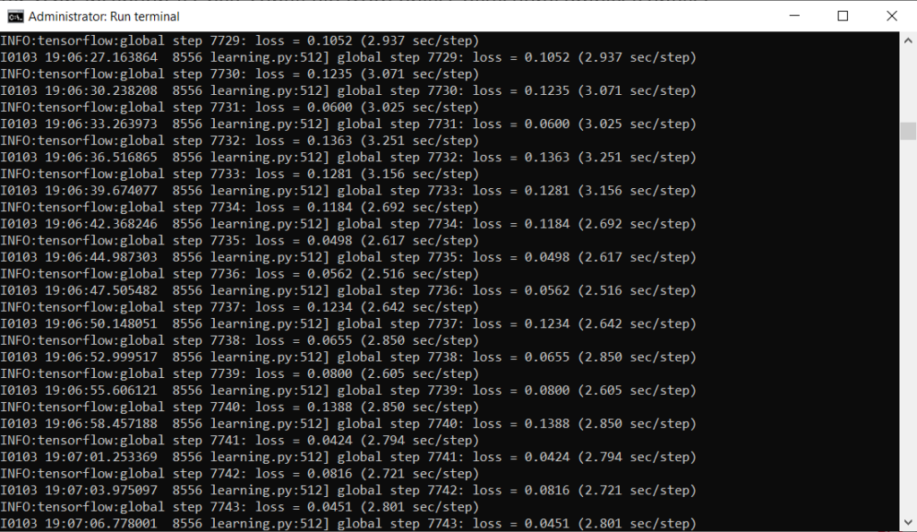
Training will take a while (about 4 hours on my laptop). You should stop when the loss consistently drops below 0.0xxx.
There is also the option of using Tensorboard and a browser as GUI if you want explained here.
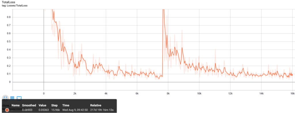
In my case I have trained so far two models. one up to 7469 iterations on 14 images (12 for training and 2 for testing) and another up to 15,961 iterations (on 30 test and 7 train images) starting from the previously trained model) with a loss of 0.0536. The new model is used for analyzing the images starting 9 August 2023 and displayed here.
The training process outputs in research/training/ several files that are named like model.ckpt-xxxx.meta. Look for the largest xxxx value. In my case it was 15961.
The final step to generate the model is to export the inference graph by issuing from a terminal the following commands (make sure you create an inference_graph folder in object_detection/):
cd C:/Users/fmarc/Downloads/models-master/models-master/research/object_detection/
python export_inference_graph.py --input_type image_tensor --pipeline_config_path training/faster_rcnn_inception_v2_pets.config --trained_checkpoint_prefix training/model.ckpt-15961 --output_directory inference_graph
This is it! Now we have a working model for our real-time solar feature detection. All it’s left is to connect the ASI120MC camera and run the image capture and ML frame analysis using our model.
Performing real-time feature detection
Real-time detection required the following:
- Adapting the code found here to work with the ASI120mc camera (and other ZWO cameras for that matter). My code can be found on github.
- Installing the zwoasi library using
pip install zwoasi - Installing the ZWO SDK.
The main issue with the existing code is that cv2 does not recognize the ZWO USB cameras. It had no issue finding the laptop camera, my 2nd USB camera, and even the OBX virtual camera, but not the ASI. For that, I had to use the zwoasi Python library and follow this tutorial.
So, here are the steps to use my code on your ZWO camera:
- Install all the required software listed at the beginning of the post plus the ZWO SDK
- Attach the ASI ZWO camera to solar scope and attach it to the computer’s USB port. Aim the h-alpha telescope at the Sun (never look at the Sun without a proper filter! It will cause permanent damage to your eyes!)
- Download the solar-ml folder from my github. Follow the instructions in the Readme file. Run the detect.py script and run it from a terminal. Assuming it is in Downloads/solar-ml/ folder the following commands (change to fit your path) will work:
cd C:/Users/fmarc/Downloads/solar-ml
python ./detect.py -gain 38 -exposure 5000
For help type: python ./detect.py -help
You can also try the detection on some recorded videos. There are test videos on my github.
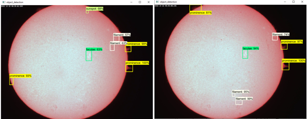
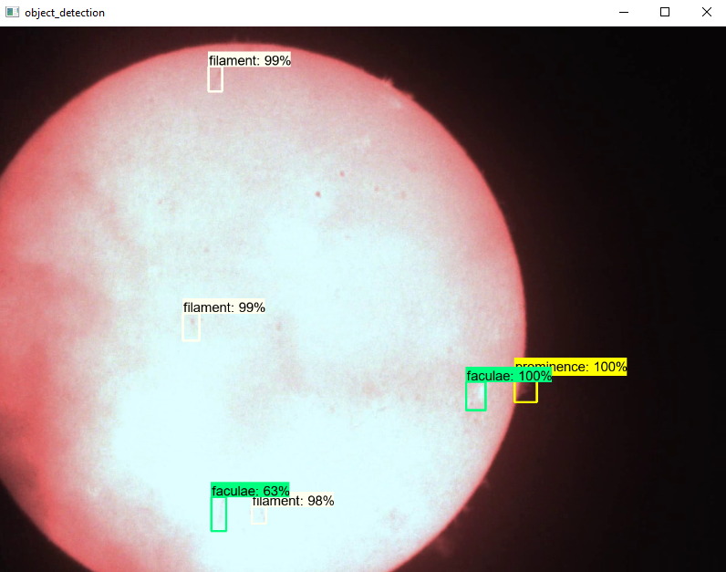
The images below show the features that the model is detecting. I admit I am impressed with the number of detections despite still having some obvious ones left out. But I reckon that is due to the small training dataset.
Tested platforms
I have tested the models on my Core i7 8th Gen Intel Laptop and on a Pi4 (armv7) board with 4GB RAM overcloaked at 2GHz. Running the live classification takes about 600 MB of memory and the liveview has an FPS=1. Yes, really low but considering that the mount I use (SkyWatcher Solarquest) tracks the Sun’s movement and that any changes in the Sun’s features usually take place at lower frequencies, this suffices for the moment. The plan is to improve the models and to reduce the memory footprint as well as to increase the FPS but the last part could require a different camera as my experiments without running the ML models (just the liveview from the camera in OpenCV) have only output up to 14 FPS on the USB 2.0 ASI120MC camera I currently use.
If you enjoyed this post consider following us on Facebook, Youtube, and Twitter or donating on Patreon. Also, stay tuned for public events Marc hosts regularly on Eventbrite.